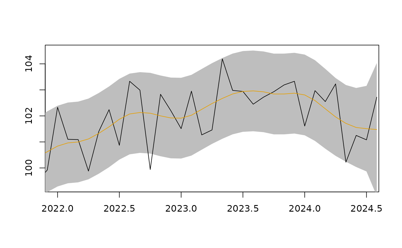
Confidence Intervals plot

Usage

confint_plot(
  object,
  xlim = NULL,
  ylim = NULL,
  col_tc = "#E69F00",
  col_sa = "black",
  col_confint = "grey",
  xlab = "",
  ylab = "",
  level = 0.95,
  ...
)

ggconfint_plot(
  object,
  xlim = NULL,
  ylim = NULL,
  col_tc = "#E69F00",
  col_sa = "black",
  col_confint = "grey",
  legend_tc = "Trend-cycle",
  legend_sa = "Seasonally adjusted",
  legend_confint = "Confidence interval",
  level = 0.95,
  ...
)

Arguments

object: "tc_estimates". The confidence intervals are computed using the confint() function.
xlim, ylim: x and y limits of the plot. If xlim is defined and not ylim, then ylim is determined automatically.
col_sa, col_tc: color of the seasonally adjusted and trend-cycle components.
col_confint: color of the confidence interval.
xlab, ylab: x and y axis labels.
level: the confidence level required.
...: other parameters.
legend_tc, legend_sa, legend_confint: legend of the trend-cycle and seasonally adjusted components and for the confidence intervals.

Examples

tc_mod <- henderson_smoothing(french_ipi[, "manufacturing"])
confint_plot(tc_mod, xlim = c(2022, 2024.5))