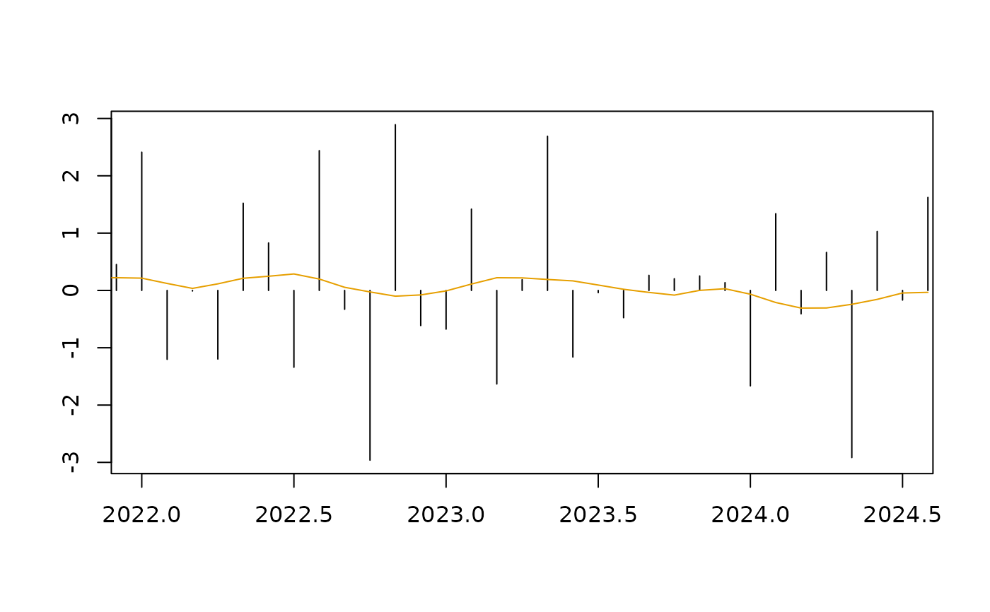
Plots the growth rate of the trend-cycle (solid lines) and the seasonally adjusted series (bar-line).
Usage
growthplot(
  object,
  pct = TRUE,
  xlim = NULL,
  ylim = NULL,
  col_tc = "#E69F00",
  col_sa = "black",
  xlab = "",
  ylab = "",
  sa_bar_line = TRUE,
  ...,
  lag = -1
)

gggrowthplot(
  object,
  pct = TRUE,
  xlim = NULL,
  ylim = NULL,
  sa_bar_line = TRUE,
  col_tc = "#E69F00",
  col_sa = "black",
  col_sa_fill = "grey",
  legend_tc = "Trend-cycle",
  legend_sa = "Seasonally adjusted",
  ...,
  lag = -1
)
Arguments
- object
"tc_estimates"object.- pct
logical. If
TRUE(the default), the growth rate is expressed in percentage points.- xlim, ylim
x and y limits of the plot. If
xlimis defined and notylim, thenylimis determined automatically.- col_sa, col_tc
color of the seasonally adjusted and trend-cycle components.
- xlab, ylab
x and y axis labels.
- sa_bar_line
logical. If
TRUE(the default), the growth rates of the seasonally adjusted series are presented as bar-lines, otherwise they are presented as lines.- ...
other (unused) parameters.
- lag
lag used for the growth rate. By default,
lag = -1(i.e. period-to-period growth rate).- col_sa_fill
fill color of the bar of the seasonally adjusted series.
- legend_tc, legend_sa
legend of the trend-cycle and seasonally adjusted components.
Examples
tc_mod <- henderson_smoothing(french_ipi[, "manufacturing"])
growthplot(tc_mod, xlim = c(2022, 2024.5))