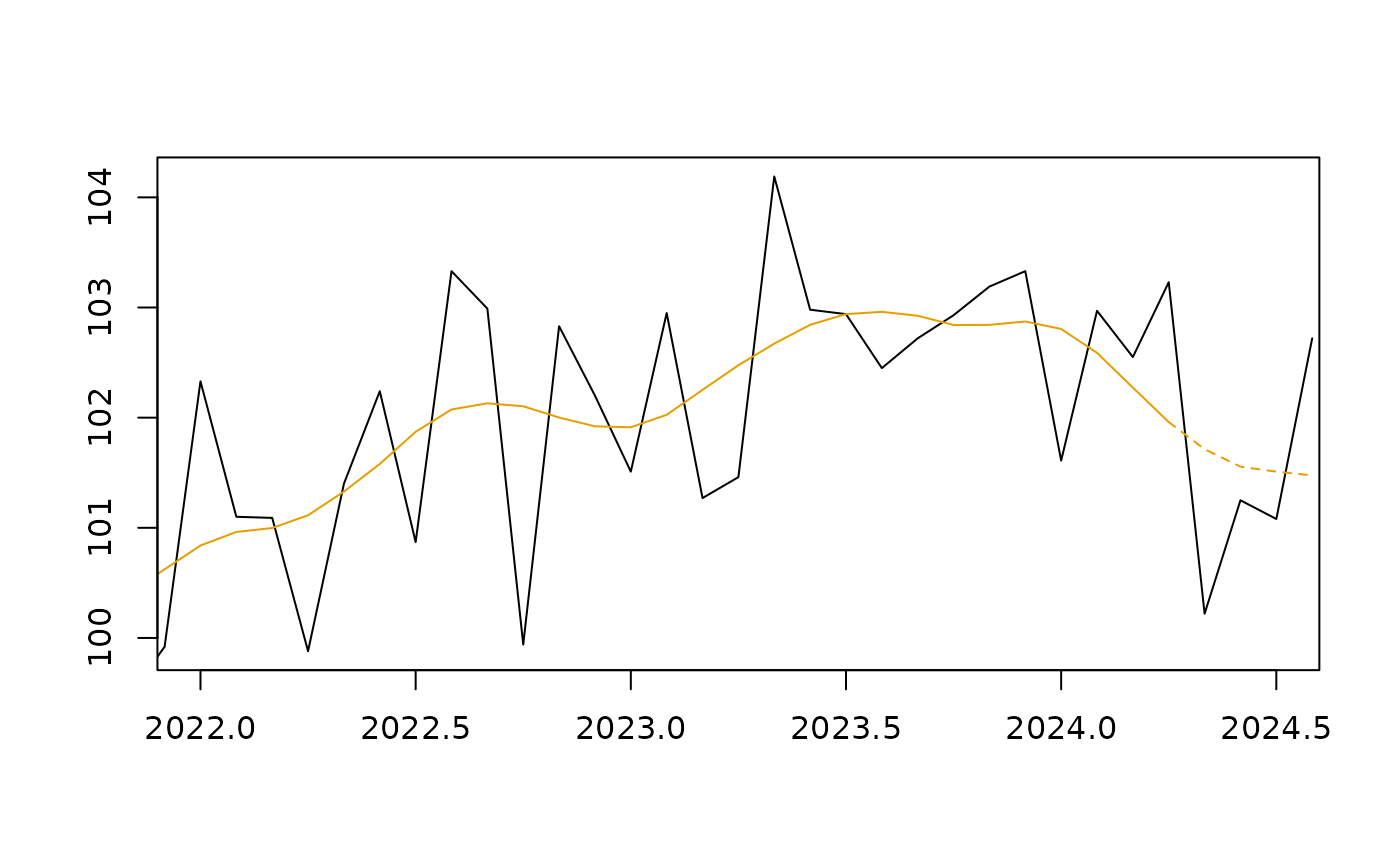
Default "tc_estimates" plot
Usage
# S3 method for class 'tc_estimates'
plot(
  x,
  y = NULL,
  xlim = NULL,
  ylim = NULL,
  col_tc = "#E69F00",
  col_sa = "black",
  xlab = "",
  ylab = "",
  lty_last_tc = 2,
  n_last_tc = 4,
  ...
)

# S3 method for class 'tc_estimates'
autoplot(
  object,
  xlim = NULL,
  ylim = NULL,
  col_tc = "#E69F00",
  col_sa = "black",
  legend_tc = "Trend-cycle",
  legend_sa = "Seasonally adjusted",
  lty_last_tc = 2,
  n_last_tc = 4,
  ...
)
Arguments
- y
unused parameter.
- xlim, ylim
x and y limits of the plot. If
xlimis defined and notylim, thenylimis determined automatically.- col_sa, col_tc
color of the seasonally adjusted and trend-cycle components.
- xlab, ylab
x and y axis labels.
- lty_last_tc
line type of the last values of the trend-cycle component.
- n_last_tc
number of last values of the trend-cycle component to be plotted with a different line type (to emphasize that there is higher variability for the last estimates). If
NULL, thenn_last_tcis equal to the MCD statistic.- ...
other (unused) parameters.
- object, x
"tc_estimates"object.- legend_tc, legend_sa
legend of the trend-cycle and seasonally adjusted components.
Examples
tc_mod <- henderson_smoothing(french_ipi[, "manufacturing"])
plot(tc_mod, xlim = c(2022, 2024.5))